14 Iterative Search

Chapter 13 demonstrated how grid search takes a pre-defined set of candidate values, evaluates them, then chooses the best settings. Iterative search methods pursue a different strategy. During the search process, they predict which values to test next.

When grid search is infeasible or inefficient, iterative methods are a sensible approach for optimizing tuning parameters.

This chapter outlines two search methods. First, we discuss Bayesian optimization, which uses a statistical model to predict better parameter settings. After that, the chapter describes a global search method called simulated annealing.

We use the same data on cell characteristics as the previous chapter for illustration, but change the model. This chapter uses a support vector machine model because it provides nice two-dimensional visualizations of the search processes.

14.1 A Support Vector Machine Model

We once again use the cell segmentation data, described in Section 13.2, for modeling, with a support vector machine (SVM) model to demonstrate sequential tuning methods. See M. Kuhn and Johnson (2013) for more information on this model. The two tuning parameters to optimize are the SVM cost value and the radial basis function kernel parameter \(\sigma\). Both parameters can have a profound effect on the model complexity and performance.

The SVM model uses a dot product and, for this reason, it is necessary to center and scale the predictors. Like the multilayer perceptron model, this model would benefit from the use of PCA feature extraction. However, we will not use this third tuning parameter in this chapter so that we can visualize the search process in two dimensions.

Along with the previously used objects (shown in Section 13.6), the tidymodels objects svm_rec, svm_spec, and svm_wflow define the model process:

library(tidymodels)
tidymodels_prefer()

svm_rec <- 
  recipe(class ~ ., data = cells) %>%
  step_YeoJohnson(all_numeric_predictors()) %>%
  step_normalize(all_numeric_predictors())

svm_spec <- 
  svm_rbf(cost = tune(), rbf_sigma = tune()) %>% 
  set_engine("kernlab") %>% 
  set_mode("classification")

svm_wflow <- 
  workflow() %>% 
  add_model(svm_spec) %>% 
  add_recipe(svm_rec)

The default parameter ranges for the two tuning parameters cost and rbf_sigma are:

cost()
#> Cost (quantitative)
#> Transformer: log-2 [1e-100, Inf]
#> Range (transformed scale): [-10, 5]
rbf_sigma()
#> Radial Basis Function sigma (quantitative)
#> Transformer: log-10 [1e-100, Inf]
#> Range (transformed scale): [-10, 0]

For illustration, let’s slightly change the kernel parameter range, to improve the visualizations of the search:

svm_param <- 
  svm_wflow %>% 
  extract_parameter_set_dials() %>% 
  update(rbf_sigma = rbf_sigma(c(-7, -1)))

Before discussing specific details about iterative search and how it works, let’s explore the relationship between the two SVM tuning parameters and the area under the ROC curve for this specific data set. We constructed a very large regular grid, composed of 2,500 candidate values, and evaluated the grid using resampling. This is obviously impractical in regular data analysis and tremendously inefficient. However, it elucidates the path that the search process should take and where the numerically optimal value(s) occur.

Figure 14.1 shows the results of evaluating this grid, with lighter color corresponding to higher (better) model performance. There is a large swath in the lower diagonal of the parameter space that is relatively flat with poor performance. A ridge of best performance occurs in the upper-right portion of the space. The black dot indicates the best settings. The transition from the plateau of poor results to the ridge of best performance is very sharp. There is also a sharp drop in the area under the ROC curve just to the right of the ridge.

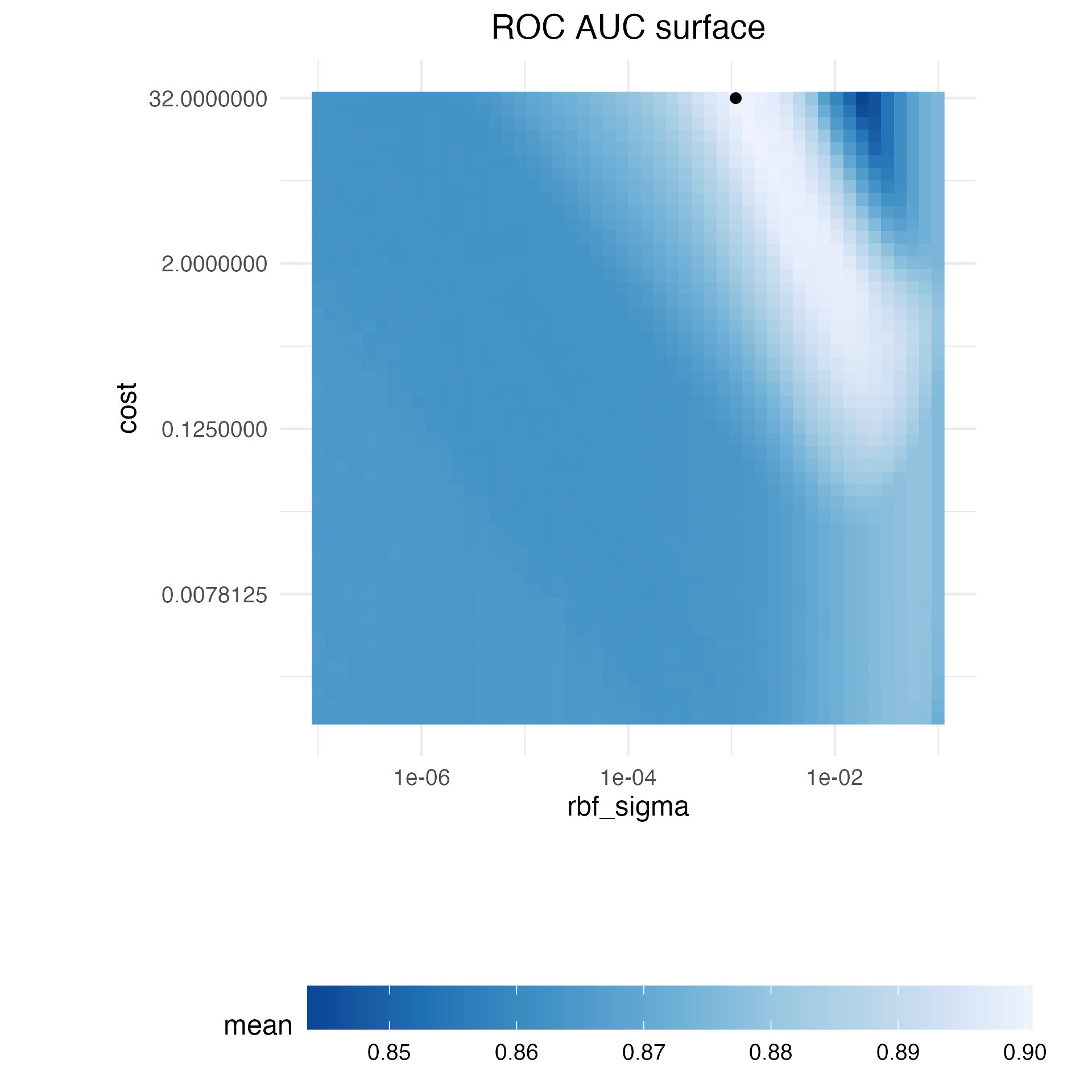
Figure 14.1: Heatmap of the mean area under the ROC curve for a high density grid of tuning parameter values. The best point is a solid dot in the upper-right corner.

The following search procedures require at least some resampled performance statistics before proceeding. For this purpose, the following code creates a small regular grid that resides in the flat portion of the parameter space. The tune_grid() function resamples this grid:

set.seed(1401)
start_grid <- 
  svm_param %>% 
  update(
    cost = cost(c(-6, 1)),
    rbf_sigma = rbf_sigma(c(-6, -4))
  ) %>% 
  grid_regular(levels = 2)

set.seed(1402)
svm_initial <- 
  svm_wflow %>% 
  tune_grid(resamples = cell_folds, grid = start_grid, metrics = roc_res)

collect_metrics(svm_initial)
#> # A tibble: 4 × 8
#>     cost rbf_sigma .metric .estimator  mean     n std_err .config             
#>    <dbl>     <dbl> <chr>   <chr>      <dbl> <int>   <dbl> <chr>               
#> 1 0.0156  0.000001 roc_auc binary     0.864    10 0.00864 Preprocessor1_Model1
#> 2 2       0.000001 roc_auc binary     0.863    10 0.00867 Preprocessor1_Model2
#> 3 0.0156  0.0001   roc_auc binary     0.863    10 0.00862 Preprocessor1_Model3
#> 4 2       0.0001   roc_auc binary     0.866    10 0.00855 Preprocessor1_Model4

This initial grid shows fairly equivalent results, with no individual point much better than any of the others. These results can be ingested by the iterative tuning functions discussed in the following sections to be used as initial values.

14.2 Bayesian Optimization

Bayesian optimization techniques analyze the current resampling results and create a predictive model to suggest tuning parameter values that have yet to be evaluated. The suggested parameter combination is then resampled. These results are then used in another predictive model that recommends more candidate values for testing, and so on. The process proceeds for a set number of iterations or until no further improvements occur. Shahriari et al. (2016) and Frazier (2018) are good introductions to Bayesian optimization.

When using Bayesian optimization, the primary concerns are how to create the model and how to select parameters recommended by that model. First, let’s consider the technique most commonly used for Bayesian optimization, the Gaussian process model.

14.2.1 A Gaussian process model

Gaussian process (GP) (Schulz, Speekenbrink, and Krause 2018) models are well-known statistical techniques that have a history in spatial statistics (under the name of kriging methods). They can be derived in multiple ways, including as a Bayesian model; see Rasmussen and Williams (2006) for an excellent reference.

Mathematically, a GP is a collection of random variables whose joint probability distribution is multivariate Gaussian. In the context of our application, this is the collection of performance metrics for the tuning parameter candidate values. For the previous initial grid of four samples, the realization of these four random variables were 0.8639, 0.8625, 0.8627, and 0.8659. These are assumed to be distributed as multivariate Gaussian. The inputs that define the independent variables/predictors for the GP model are the corresponding tuning parameter values (shown in Table 14.1).

Table 14.1: Resampling statistics used as the initial substrate to the Gaussian process model.

outcome	predictors
ROC	cost	rbf_sigma
0.8639	0.01562	0.000001
0.8625	2.00000	0.000001
0.8627	0.01562	0.000100
0.8659	2.00000	0.000100

Gaussian process models are specified by their mean and covariance functions, although the latter has the most effect on the nature of the GP model. The covariance function is often parameterized in terms of the input values (denoted as \(x\)). As an example, a commonly used covariance function is the squared exponential³⁰ function:

\[\operatorname{cov}(\boldsymbol{x}_i, \boldsymbol{x}_j) = \exp\left(-\frac{1}{2}|\boldsymbol{x}_i - \boldsymbol{x}_j|^2\right) + \sigma^2_{ij}\] where \(\sigma^2_{ij}\) is a constant error variance term that is zero when \(i=j\). This equation translates to:

As the distance between two tuning parameter combinations increases, the covariance between the performance metrics increase exponentially.

The nature of the equation also implies that the variation of the outcome metric is minimized at the points that have already been observed (i.e., when \(|\boldsymbol{x}_i - \boldsymbol{x}_j|^2\) is zero).

The nature of this covariance function allows the Gaussian process to represent highly nonlinear relationships between model performance and the tuning parameters even when only a small amount of data exists.

However, fitting these models can be difficult in some cases, and the model becomes more computationally expensive as the number of tuning parameter combinations increases.

An important virtue of this model is that, since a full probability model is specified, the predictions for new inputs can reflect the entire distribution of the outcome. In other words, new performance statistics can be predicted in terms of both mean and variance.

Suppose that two new tuning parameters were under consideration. In Table 14.2, candidate A has a slightly better mean ROC value than candidate B (the current best is 0.8659). However, its variance is four-fold larger than B. Is this good or bad? Choosing option A is riskier but has potentially higher return. The increase in variance also reflects that this new value is farther from the existing data than B. The next section considers these aspects of GP predictions for Bayesian optimization in more detail.

Table 14.2: Two example tuning parameters considered for further sampling.

	GP Prediction of ROC AUC
candidate	mean	variance
A	0.90	0.000400
B	0.89	0.000025

Bayesian optimization is an iterative process.

Based on the initial grid of four results, the GP model is fit, candidates are predicted, and a fifth tuning parameter combination is selected. We compute performance estimates for the new configuration, the GP is refit with the five existing results (and so on).

14.2.2 Acquisition functions

Once the Gaussian process is fit to the current data, how is it used? Our goal is to choose the next tuning parameter combination that is most likely to have “better results” than the current best. One approach to do this is to create a large candidate set (perhaps using a space-filling design) and then make mean and variance predictions on each. Using this information, we choose the most advantageous tuning parameter value.

A class of objective functions, called acquisition functions, facilitate the trade-off between mean and variance. Recall that the predicted variance of the GP models are mostly driven by how far away they are from the existing data. The trade-off between the predicted mean and variance for new candidates is frequently viewed through the lens of exploration and exploitation:

• Exploration biases the selection towards regions where there are fewer (if any) observed candidate models. This tends to give more weight to candidates with higher variance and focuses on finding new results.

• Exploitation principally relies on the mean prediction to find the best (mean) value. It focuses on existing results.

To demonstrate, let’s look at a toy example with a single parameter that has values between [0, 1] and the performance metric is \(R^2\). The true function is shown in Figure 14.2, along with five candidate values that have existing results as points.

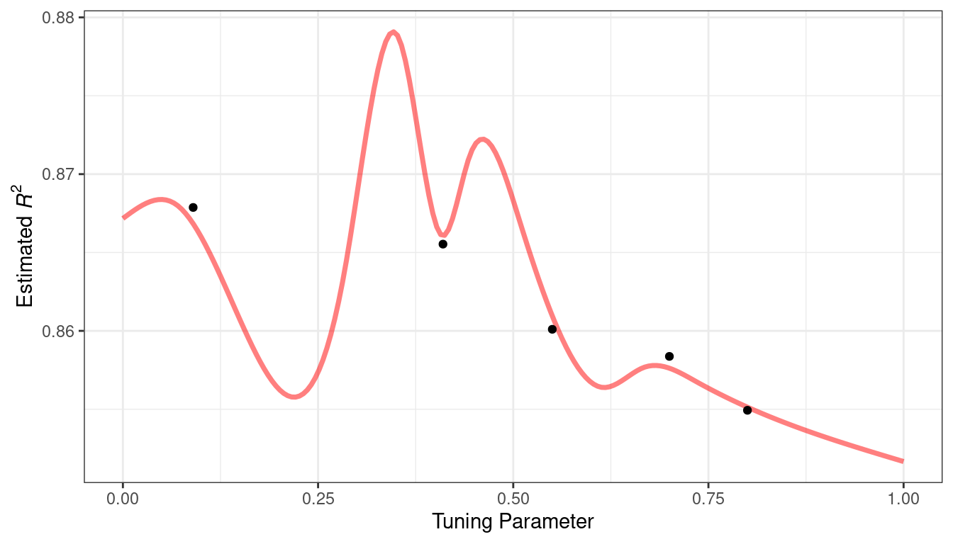
Figure 14.2: Hypothetical true performance profile over an arbitrary tuning parameter, with five estimated points

For these data, the GP model fit is shown in Figure 14.3. The shaded region indicates the mean \(\pm\) 1 standard error. The two vertical lines indicate two candidate points that are examined in more detail later.

The shaded confidence region demonstrates the squared exponential variance function; it becomes very large between points and converges to zero at the existing data points.

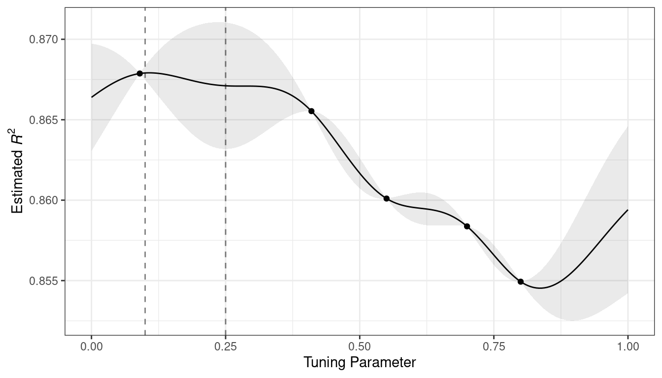
Figure 14.3: Estimated performance profile generated by the Gaussian process model. The shaded region shows one-standard-error bounds.

This nonlinear trend passes through each observed point, but the model is not perfect. There are no observed points near the true optimum setting and, in this region, the fit could be much better. Despite this, the GP model can effectively point us in the right direction.

From a pure exploitation standpoint, the best choice would select the parameter value that has the best mean prediction. Here, this would be a value of 0.106, just to the right of the existing best observed point at 0.09.

As a way to encourage exploration, a simple (but not often used) approach is to find the tuning parameter associated with the largest confidence interval. For example, by using a single standard deviation for the \(R^2\) confidence bound, the next point to sample would be 0.236. This is slightly more into the region with no observed results. Increasing the number of standard deviations used in the upper bound would push the selection farther into empty regions.

One of the most commonly used acquisition functions is expected improvement. The notion of improvement requires a value for the current best results (unlike the confidence bound approach). Since the GP can describe a new candidate point using a distribution, we can weight the parts of the distribution that show improvement using the probability of the improvement occurring.

For example, consider two candidate parameter values of 0.10 and 0.25 (indicated by the vertical lines in Figure 14.3). Using the fitted GP model, their predicted \(R^2\) distributions are shown in Figure 14.4 along with a reference line for the current best results.

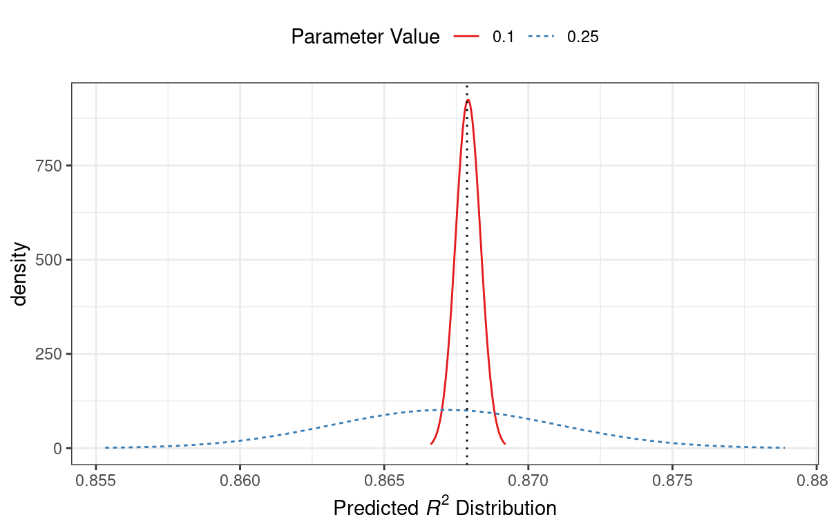
Figure 14.4: Predicted performance distributions for two sampled tuning parameter values

When only considering the mean \(R^2\) prediction, a parameter value of 0.10 is the better choice (see Table 14.3). The tuning parameter recommendation for 0.25 is, on average, predicted to be worse than the current best. However, since it has higher variance, it has more overall probability area above the current best. As a result, it has a larger expected improvement:

Table 14.3: Expected improvement for the two candidate tuning parameters.

	Predictions
Parameter Value	Mean	Std Dev	Expected Improvment
0.10	0.8679	0.0004317	0.000190
0.25	0.8671	0.0039301	0.001216

When expected improvement is computed across the range of the tuning parameter, the recommended point to sample is much closer to 0.25 than 0.10, as shown in Figure 14.5.

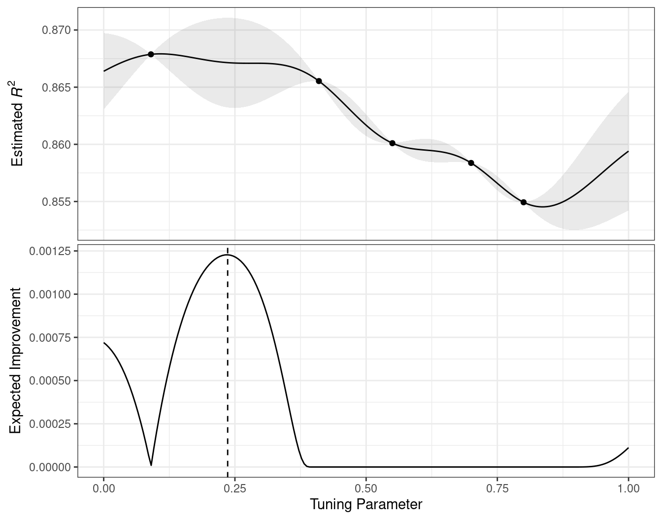
Figure 14.5: The estimated performance profile generated by the Gaussian process model (top panel) and the expected improvement (bottom panel). The vertical line indicates the point of maximum improvement.

Numerous acquisition functions have been proposed and discussed; in tidymodels, expected improvement is the default.

14.2.3 The tune_bayes() function

To implement iterative search via Bayesian optimization, use the tune_bayes() function. Its syntax is very similar to tune_grid() but with several additional arguments:

• iter is the maximum number of search iterations.

• initial can be either an integer, an object produced using tune_grid(), or one of the racing functions. Using an integer specifies the size of a space-filling design that is sampled prior to the first GP model.

• objective is an argument for which acquisition function should be used. The tune package contains functions to pass here, such as exp_improve() or conf_bound().

• The param_info argument, in this case, specifies the range of the parameters as well as any transformations that are used. These are used to define the search space. In situations where the default parameter objects are insufficient, param_info is used to override the defaults.

The control argument now uses the results of control_bayes(). Some helpful arguments there are:

• no_improve is an integer that will stop the search if improved parameters are not discovered within no_improve iterations.

• uncertain is also an integer (or Inf) that will take an uncertainty sample if there is no improvement within uncertain iterations. This will select the next candidate that has large variation. It has the effect of pure exploration since it does not consider the mean prediction.

• verbose is a logical that will print logging information as the search proceeds.

Let’s use the first SVM results from Section 14.1 as the initial substrate for the Gaussian process model. Recall that, for this application, we want to maximize the area under the ROC curve. Our code is:

ctrl <- control_bayes(verbose = TRUE)

set.seed(1403)
svm_bo <-
  svm_wflow %>%
  tune_bayes(
    resamples = cell_folds,
    metrics = roc_res,
    initial = svm_initial,
    param_info = svm_param,
    iter = 25,
    control = ctrl
  )

The search process starts with an initial best value of 0.8659 for the area under the ROC curve. A Gaussian process model uses these four statistics to create a model. The large candidate set is automatically generated and scored using the expected improvement acquisition function. The first iteration failed to improve the outcome with an ROC value of 0.86315. After fitting another Gaussian process model with the new outcome value, the second iteration also failed to yield an improvement.

The log of the first two iterations, produced by the verbose option, was:

The search continues. There were a total of 9 improvements in the outcome along the way at iterations 3, 4, 5, 6, 8, 13, 22, 23, and 24. The best result occurred at iteration 24 with an area under the ROC curve of 0.8986.

The last step was:

The functions that are used to interrogate the results are the same as those used for grid search (e.g., collect_metrics(), etc.). For example:

show_best(svm_bo)
#> # A tibble: 5 × 9
#>    cost rbf_sigma .metric .estimator  mean     n std_err .config .iter
#>   <dbl>     <dbl> <chr>   <chr>      <dbl> <int>   <dbl> <chr>   <int>
#> 1  31.8   0.00160 roc_auc binary     0.899    10 0.00785 Iter24     24
#> 2  30.8   0.00191 roc_auc binary     0.899    10 0.00791 Iter23     23
#> 3  31.4   0.00166 roc_auc binary     0.899    10 0.00784 Iter22     22
#> 4  31.8   0.00153 roc_auc binary     0.899    10 0.00783 Iter13     13
#> 5  30.8   0.00163 roc_auc binary     0.899    10 0.00782 Iter15     15

The autoplot() function has several options for iterative search methods. Figure 14.6 shows how the outcome changed over the search by using autoplot(svm_bo, type = "performance").

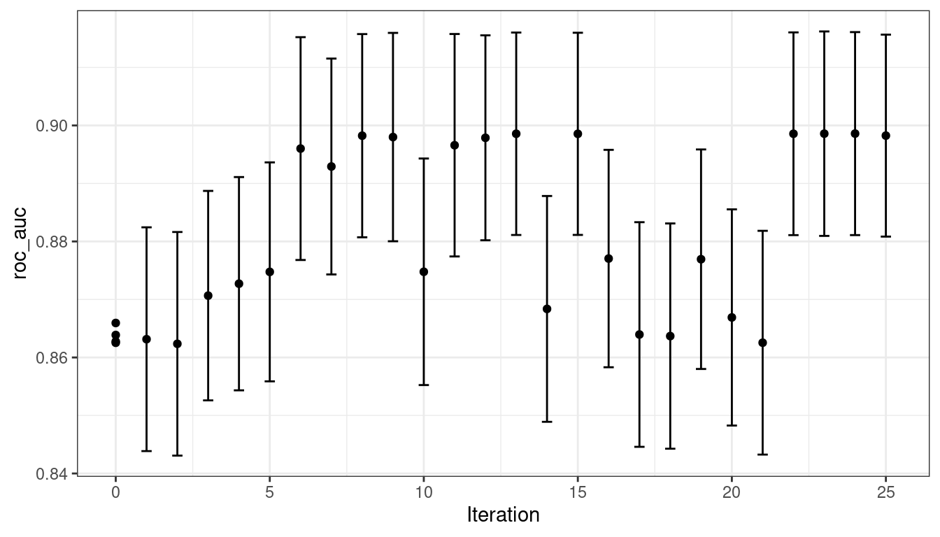
Figure 14.6: The progress of the Bayesian optimization produced when the autoplot() method is used with type = "performance"

An additional type of plot uses type = "parameters" that shows the parameter values over iterations.

The animation below visualizes the results of the search. The black \(\times\) values show the starting values contained in svm_initial. The top-left blue panel shows the predicted mean value of the area under the ROC curve. The red panel on the top-right displays the predicted variation in the ROC values while the bottom plot visualizes the expected improvement. In each panel, darker colors indicate less attractive values (e.g., small mean values, large variation, and small improvements).

The surface of the predicted mean surface is very inaccurate in the first few iterations of the search. Despite this, it does help guide the process to the region of good performance. In other words, the Gaussian process model is wrong but shows itself to be very useful. Within the first ten iterations, the search is sampling near the optimum location.

While the best tuning parameter combination is on the boundary of the parameter space, Bayesian optimization will often choose new points on other sides of the boundary. While we can adjust the ratio of exploration and exploitation, the search tends to sample boundary points early on.

If the search is seeded with an initial grid, a space-filling design would probably be a better choice than a regular design. It samples more unique values of the parameter space and would improve the predictions of the standard deviation in the early iterations.

Finally, if the user interrupts the tune_bayes() computations, the function returns the current results (instead of resulting in an error).

14.3 Simulated Annealing

Simulated annealing (SA) (Kirkpatrick, Gelatt, and Vecchi 1983; Van Laarhoven and Aarts 1987) is a general nonlinear search routine inspired by the process in which metal cools. It is a global search method that can effectively navigate many different types of search landscapes, including discontinuous functions. Unlike most gradient-based optimization routines, simulated annealing can reassess previous solutions.

14.3.1 Simulated annealing search process

The process of using simulated annealing starts with an initial value and embarks on a controlled random walk through the parameter space. Each new candidate parameter value is a small perturbation of the previous value that keeps the new point within a local neighborhood.

The candidate point is resampled to obtain its corresponding performance value. If this achieves better results than the previous parameters, it is accepted as the new best and the process continues. If the results are worse than the previous value the search procedure may still use this parameter to define further steps. This depends on two factors. First, the likelihood of accepting a bad result decreases as performance becomes worse. In other words, a slightly worse result has a better chance of acceptance than one with a large drop in performance. The other factor is the number of search iterations. Simulated annealing wants to accept fewer suboptimal values as the search proceeds. From these two factors, the acceptance probability for a bad result can be formalized as:

\[\operatorname{Pr}[\text{accept suboptimal parameters at iteration } i] = \exp(c\times D_i \times i)\]

where \(i\) is the iteration number, \(c\) is a user-specified constant, and \(D_i\) is the percent difference between the old and new values (where negative values imply worse results). For a bad result, we determine the acceptance probability and compare it to a random uniform number. If the random number is greater than the probability value, the search discards the current parameters and the next iteration creates its candidate value in the neighborhood of the previous value. Otherwise, the next iteration forms the next set of parameters based on the current (suboptimal) values.

The acceptance probabilities of simulated annealing allow the search to proceed in the wrong direction, at least for the short term, with the potential to find a much better region of the parameter space in the long run.

How are the acceptance probabilities influenced? The heatmap in Figure 14.7 shows how the acceptance probability can change over iterations, performance, and the user-specified coefficient.

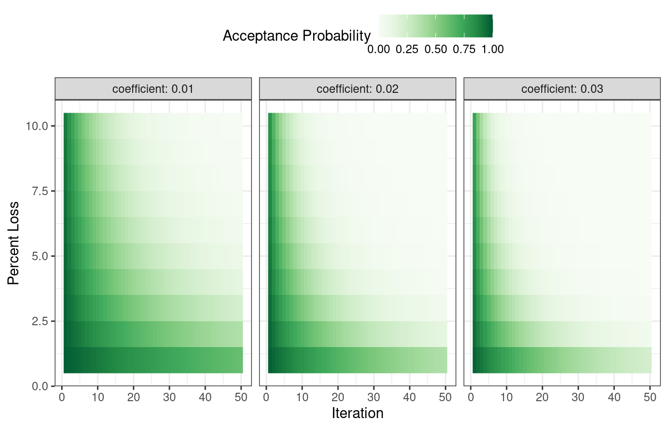
Figure 14.7: Heatmap of the simulated annealing acceptance probabilities for different coefficient values

The user can adjust the coefficients to find a probability profile that suits their needs. In finetune::control_sim_anneal(), the default for this cooling_coef argument is 0.02. Decreasing this coefficient will encourage the search to be more forgiving of poor results.

This process continues for a set amount of iterations but can halt if no globally best results occur within a pre-determined number of iterations. However, it can be very helpful to set a restart threshold. If there are a string of failures, this feature revisits the last globally best parameter settings and starts anew.

The main important detail is to define how to perturb the tuning parameters from iteration to iteration. There are a variety of methods in the literature for this. We follow the method given in Bohachevsky, Johnson, and Stein (1986) called generalized simulated annealing. For continuous tuning parameters, we define a small radius to specify the local “neighborhood.” For example, suppose there are two tuning parameters and each is bounded by zero and one. The simulated annealing process generates random values on the surrounding radius and randomly chooses one to be the current candidate value.

In our implementation, the neighborhood is determined by scaling the current candidate to be between zero and one based on the range of the parameter object, so radius values between 0.05 and 0.15 seem reasonable. For these values, the fastest that the search could go from one side of the parameter space to the other is about 10 iterations. The size of the radius controls how quickly the search explores the parameter space. In our implementation, a range of radii is specified so different magnitudes of “local” define the new candidate values.

To illustrate, we’ll use the two main glmnet tuning parameters:

• The amount of total regularization (penalty). The default range for this parameter is \(10^{-10}\) to \(10^{0}\). It is typical to use a log (base-10) transformation for this parameter.

• The proportion of the lasso penalty (mixture). This is bounded at zero and one with no transformation.

The process starts with initial values of penalty = 0.025 and mixture = 0.050. Using a radius that randomly fluctuates between 0.050 and 0.015, the data are appropriately scaled, random values are generated on radii around the initial point, then one is randomly chosen as the candidate. For illustration, we will assume that all candidate values are improvements. Using the new value, a set of new random neighbors are generated, one is chosen, and so on. Figure 14.8 shows six iterations as the search proceeds toward the upper left corner.

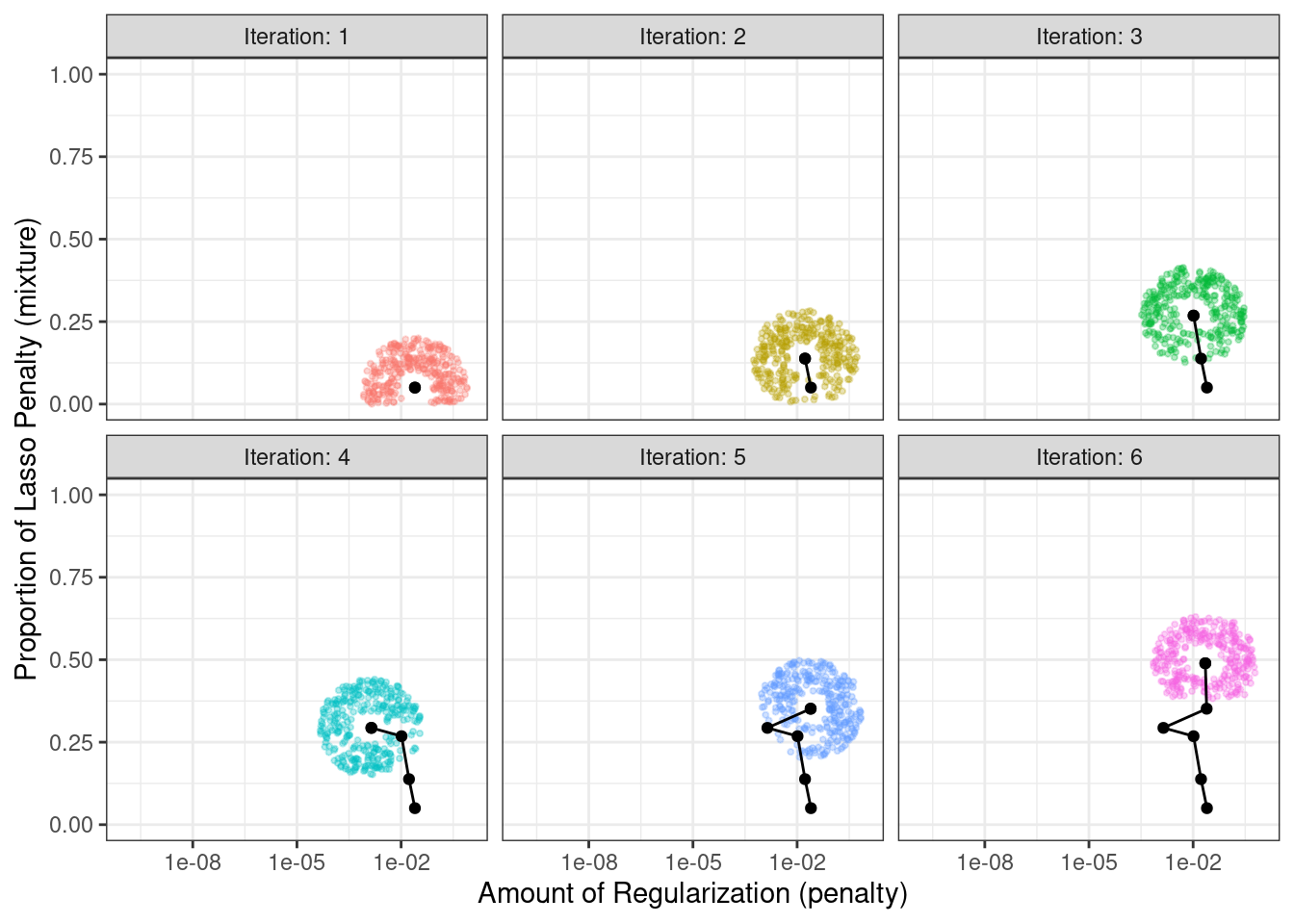
Figure 14.8: An illustration of how simulated annealing determines what is the local neighborhood for two numeric tuning parameters. The clouds of points show possible next values where one would be selected at random.

Note that, during some iterations, the candidate sets along the radius exclude points outside of the parameter boundaries. Also, our implementation biases the choice of the next tuning parameter configurations away from new values that are very similar to previous configurations.

For non-numeric parameters, we assign a probability for how often the parameter value changes.

14.3.2 The tune_sim_anneal() function

To implement iterative search via simulated annealing, use the tune_sim_anneal() function. The syntax for this function is nearly identical to tune_bayes(). There are no options for acquisition functions or uncertainty sampling. The control_sim_anneal() function has some details that define the local neighborhood and the cooling schedule:

• no_improve, for simulated annealing, is an integer that will stop the search if no global best or improved results are discovered within no_improve iterations. Accepted suboptimal or discarded parameters count as “no improvement.”

• restart is the number of iterations with no new best results before starting from the previous best results.

• radius is a numeric vector on (0, 1) that defines the minimum and maximum radius of the local neighborhood around the initial point.

• flip is a probability value that defines the chances of altering the value of categorical or integer parameters.

• cooling_coef is the \(c\) coefficient in \(\exp(c\times D_i \times i)\) that modulates how quickly the acceptance probability decreases over iterations. Larger values of cooling_coef decrease the probability of accepting a suboptimal parameter setting.

For the cell segmentation data, the syntax is very consistent with the previously used functions:

ctrl_sa <- control_sim_anneal(verbose = TRUE, no_improve = 10L)

set.seed(1404)
svm_sa <-
  svm_wflow %>%
  tune_sim_anneal(
    resamples = cell_folds,
    metrics = roc_res,
    initial = svm_initial,
    param_info = svm_param,
    iter = 50,
    control = ctrl_sa
  )

The simulated annealing process discovered new global optimums at 4 different iterations. The earliest improvement was at iteration 5 and the final optimum occured at iteration 27. The best overall results occured at iteration 27 with a mean area under the ROC curve of 0.8985 (compared to an initial best of 0.8659). There were 4 restarts at iterations 13, 21, 35, and 43 as well as 12 discarded candidates during the process.

The verbose option prints details of the search process. The output for the first five iterations was:

The output for last ten iterations was:

#> 40 ◯ accept suboptimal  roc_auc=0.89606 (+/-0.008203)
#> 
#> 41 ─ discard suboptimal roc_auc=0.87556 (+/-0.009272)
#> 
#> 42 ─ discard suboptimal roc_auc=0.87198 (+/-0.009301)
#> 
#> 43 ✖ restart from best  roc_auc=0.89801 (+/-0.008224)
#> 
#> 44 ◯ accept suboptimal  roc_auc=0.89006 (+/-0.008789)
#> 
#> 45 + better suboptimal  roc_auc=0.89781 (+/-0.008104)
#> 
#> 46 ◯ accept suboptimal  roc_auc=0.89563 (+/-0.008601)
#> 
#> 47 ─ discard suboptimal roc_auc=0.88527 (+/-0.008766)
#> 
#> 48 ◯ accept suboptimal  roc_auc=0.8922 (+/-0.008891)
#> 
#> 49 ─ discard suboptimal roc_auc=0.87691 (+/-0.008352)
#> 
#> 50 ◯ accept suboptimal  roc_auc=0.88803 (+/-0.008728)

As with the other tune_*() functions, the corresponding autoplot() function produces visual assessments of the results. Using autoplot(svm_sa, type = "performance") shows the performance over iterations (Figure 14.9) while autoplot(svm_sa, type = "parameters") plots performance versus specific tuning parameter values (Figure 14.10).

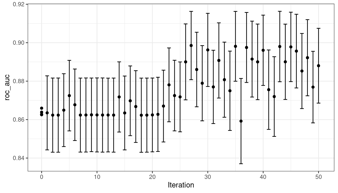
Figure 14.9: Progress of the simulated annealing process shown when the autoplot() method is used with type = "performance"

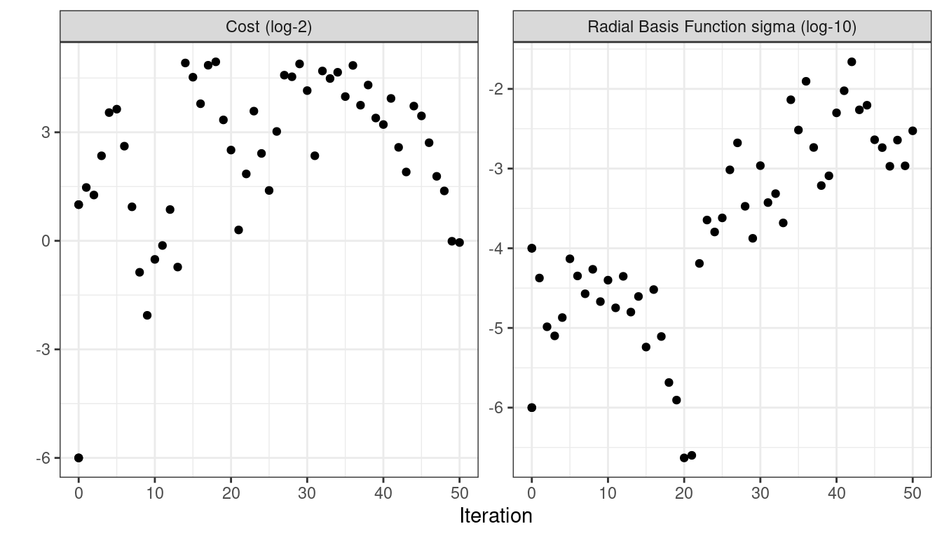
Figure 14.10: Performance versus tuning parameter values when the autoplot() method is used with type = "parameters".

A visualization of the search path helps to understand where the search process did well and where it went astray:

Like tune_bayes(), manually stopping execution will return the completed iterations.

14.4 Chapter Summary

This chapter described two iterative search methods for optimizing tuning parameters. Bayes optimization uses a predictive model trained on existing resampling results to suggest tuning parameter values, while simulated annealing walks through the hyperparameter space to find good values. Both can be effective at finding good values alone or as a follow-up method used after an initial grid search to further finetune performance.

REFERENCES

Bohachevsky, I, M Johnson, and M Stein. 1986. “Generalized Simulated Annealing for Function Optimization.” Technometrics 28 (3): 209–17.

Frazier, R. 2018. “A Tutorial on Bayesian Optimization.” https://arxiv.org/abs/1807.02811.

Kirkpatrick, S, D Gelatt, and M Vecchi. 1983. “Optimization by Simulated Annealing.” Science 220 (4598): 671–80.

Kuhn, M, and K Johnson. 2013. Applied Predictive Modeling. Springer.

Rasmussen, C, and C Williams. 2006. Gaussian Processes for Machine Learning. Gaussian Processes for Machine Learning. MIT Press.

Schulz, E, M Speekenbrink, and A Krause. 2018. “A Tutorial on Gaussian Process Regression: Modelling, Exploring, and Exploiting Functions.” Journal of Mathematical Psychology 85: 1–16.

Shahriari, B., K. Swersky, Z. Wang, R. P. Adams, and N. de Freitas. 2016. “Taking the Human Out of the Loop: A Review of Bayesian Optimization.” Proceedings of the IEEE 104 (1): 148–75.

Van Laarhoven, P, and E Aarts. 1987. “Simulated Annealing.” In Simulated Annealing: Theory and Applications, 7–15. Springer.

---

30. This equation is also the same as the radial basis function used in kernel methods, such as the SVM model that is currently being used. This is a coincidence; this covariance function is unrelated to the SVM tuning parameter that we are using. ↩︎